Discrete Callback

Ian Wineman

Discrete Callback for a simple neuron model

Published: Dec 26, '24; Last Updated: Dec 26, '24.

There are several examples provided of discrete callback in the documentation for DifferentialEquations.jl, but here we provide an additional example from computational neuroscience.

Izhikevich presents a “simple model” of a neuron in his Dynamical Systems in Neuroscience (see also here).

...

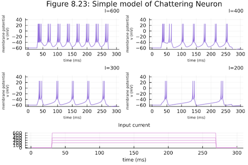
The model is simple because it is only a two dimensional model, and yet, for certain parameters, can exhibit behaviors seen in higher dimensional models (and real neurons), like spiking, bursting, and chattering. The simple model is amenable to many geometric methods of analysis, since its phase space can be represented as a plane. Another benefit of such a simple model, is that it is far less computational intensive to simulate, which is beneficial when simulating a large collection of neurons.

Simple model of chattering neuron — *Simple model of a chattering neuron; reproduced from Izhikevich 2007, Figure 8.23, page 295; source code.*

The primary difference between the simple model and a traditional two dimensional dynamical system is the resetting behavior when v >= vpeak. This behavior can be easily implemented into a solver using the Discrete Callback functionality within DifferentialEquations.jl.

We will walk through the example piece by piece, or you can skip ahead to the full example.

First, we specify the model itself with given values for the free parameters of the model. The parameters are chosen to simulate a neuron from a cat primary visual cortex.

global vpeak = 35

function model!(du, u, p, t)
    C,vr,vt,k=[100,-60,-40,0.7]
    a,b=[0.03,-2]
    I = p
    du[1] = (I(t) + k * (u[1] - vr) * (u[1] - vt) - u[2]) / C
    du[2] = a * (b * (u[1] - vr) - u[2])
end

Next, we specify the condition for the reset and its affect.

function vpeak_check(u, t, integrator)
    u[1] ≥ vpeak
end

function affect!(integrator)
    c, d = [-50,100]
    integrator.u[1] = c
    integrator.u[2] += d
end

Finally, we set up the problem and solve it.

cb = DiscreteCallback(vpeak_check, affect!)
cbs = CallbackSet(cb)

vr=-60
u0=[vr,0]
p(t)=t<100 ? 0 : 70 # injected DC current
prob = ODEProblem(model!, u0, (0.0, 1000.0), p)

sol = solve(prob, Tsit5(), callback = cbs)

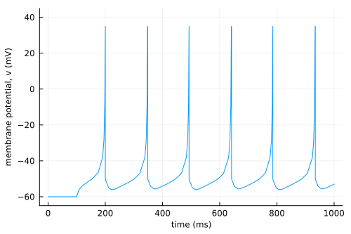
Plotting the solution we can see the spiking behavior of the neuron model.

plot(
    sol.t,
    [i≥35 ? vpeak : i for i=sol[1, :]],
    ylim=[-65,45],
    xtick=0:200:1000,
    ytick=-60:20:40,
    label="",
    xlabel="time (ms)",
    ylabel="membrane potential, v (mV)",
    xguidefontsize=8,
    yguidefontsize=8
)

Full Example

using Plots, DifferentialEquations

global vpeak = 35

function model!(du, u, p, t)
    C,vr,vt,k=[100,-60,-40,0.7]
    a,b=[0.03,-2]
    I = p
    du[1] = (I(t) + k * (u[1] - vr) * (u[1] - vt) - u[2]) / C
    du[2] = a * (b * (u[1] - vr) - u[2])
end

function vpeak_check(u, t, integrator)
    u[1] ≥ vpeak
end

function affect!(integrator)
    c, d = [-50,100]
    integrator.u[1] = c
    integrator.u[2] += d
end

cb = DiscreteCallback(vpeak_check, affect!)
cbs = CallbackSet(cb)

vr=-60
u0=[vr,0]
p(t)=t<100 ? 0 : 70 # injected DC current
prob = ODEProblem(model!, u0, (0.0, 1000.0), p)

sol = solve(prob, Tsit5(), callback = cbs)

plot(
    sol.t,
    [i≥35 ? vpeak : i for i=sol[1, :]],
    ylim=[-65,45],
    xtick=0:200:1000,
    ytick=-60:20:40,
    label="",
    xlabel="time (ms)",
    ylabel="membrane potential, v (mV)",
    xguidefontsize=8,
    yguidefontsize=8
)